DVP-IO x SOPA/Cellpose

In this tutorial, we will run the cell segmentation pipeline implemented in sopa [BMG+24] to perform cell segmentation of a multi-channel fluorescence image in the .czi format with cellpose. We will use dvp-io to read the image from its native format into the sopa-supported spatialdata format. Subsequently, we will run the sopa cell segmentation pipeline. Finally we will use dvp-io to export the shapes as LMD-compatible .xml file.

Load modules

This tutorial requires you to have sopa with cellpose support installed in your local environment.

conda create -n dvpio python=3.11 -y && conda activate dvpio
pip install dvp-io
pip install "sopa[cellpose]"

import sopa
from dvpio.read.image import read_czi
from dvpio.write.shapes import write_lmd
import spatialdata_plot  # noqa
import spatialdata as sd
import numpy as np
import matplotlib.pyplot as plt

Load data

We will use a sample .czi image (3 channels) kindly provided by Sophia Mädler from the scPortrait package [SMW+23] and convert it to a spatialdata object using dvpio.read.image.read_czi. Note that the converted spatialdata object must be written to disk for the rest of the notebook to function. This is because some features of read_czi rely on C modules that cannot be parallelized by Dask, which sopa’s parallelization backend depends on.

## Uncomment to obtain data
# ! wget -O "./data/example.czi" "https://datashare.biochem.mpg.de/s/4jH87DiwvxoM4Qd/download"

sdata = sd.SpatialData()

# Get all 3 channels from czi image
sdata.images["czi"] = read_czi("./data/example.czi", channels=[0, 1, 2])

# Write sdata to disk
sdata.write("./data/scportrait-czi.sdata.zarr")

INFO     The Zarr backing store has been changed from None the new file path: data/scportrait-czi.sdata.zarr

# Re-read sdata object from disk
sdata = sd.read_zarr("./data/scportrait-czi.sdata.zarr")

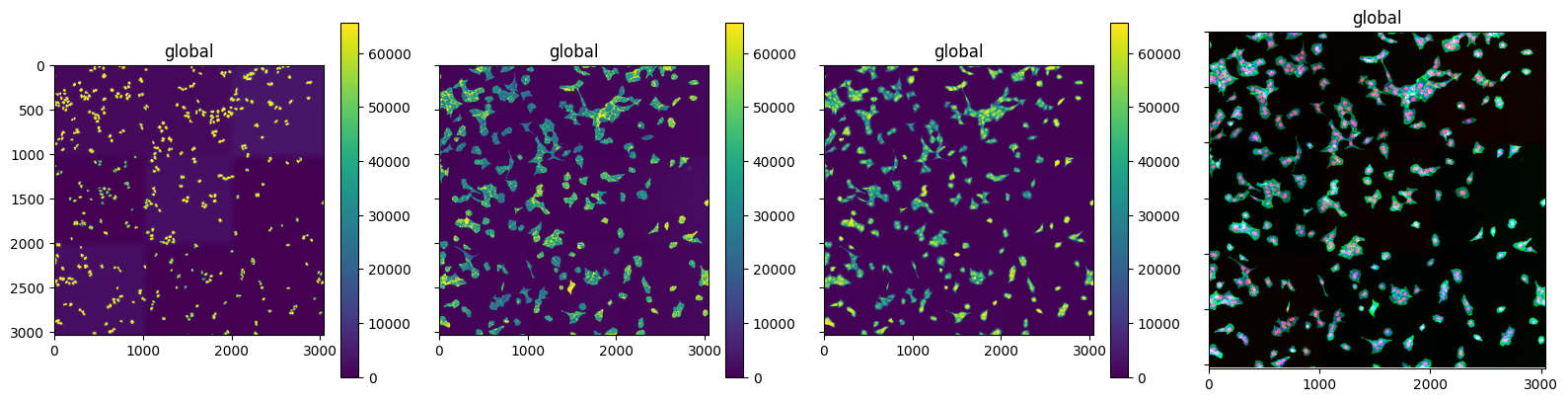
We can plot the 3 channels. Channel 0 corresponds to the nuclei channel and 1 to the cytosol channel

fig, axs = plt.subplots(1, 4, figsize=(16, 4), sharex=True, sharey=True)

for idx in range(3):
    sdata.pl.render_images("czi", channel=idx).pl.show(ax=axs[idx])


sdata.pl.render_images("czi").pl.show(ax=axs[3])
plt.tight_layout()

INFO     Rasterizing image for faster rendering.                                                                   
INFO     Rasterizing image for faster rendering.                                                                   
INFO     Rasterizing image for faster rendering.                                                                   
INFO     Rasterizing image for faster rendering.

Run sopa

We can now run sopa. Sopa first creates smaller image patches that can be passed to cellpose, using the sopa.make_image_patches method. Subsquently, we can run the cellpose wrapper sopa.segmentation.cellpose. Note that you can also pass your own pretrained models to via the pretrained_model="/path/to/pretrained/model" argument. Here, we are using the default cyto3 model.

sopa.make_image_patches(sdata, patch_width=500, patch_overlap=50, image_key="czi")

# Set dask as parallelization backend
sopa.settings.parallelization_backend = "dask"

sopa.segmentation.cellpose(sdata, channels=[1, 0], diameter=50, model_type="cyto3", image_key="czi")

# Runs in ca. 30s on MacOS/M3

[                                        ] | 0% Completed |  0.4s
[########################################] | 100% Completed | 23.3s

We can inspect the cell segmentation in a smaller patch and we can see that the model performed well on this dataset.

(
    sdata.query.bounding_box(
        axes=("x", "y"),
        min_coordinate=np.array([0, 0]),
        max_coordinate=np.array([600, 600]),
        target_coordinate_system="global",
    )
    .pl.render_images("czi")
    .pl.render_shapes("cellpose_boundaries", fill_alpha=0, outline_alpha=1)
    .pl.show()
)

Write shapes

In many cases, we are now interested in exporting the obtained shapes to a Leica Microdissection Microscope. We can use the dvpio.write.write_lmd function to export shapes in a compatible format. The function wraps the py-LMD package [SMW+23].

The function also relies on adding calibration points

sdata

SpatialData object, with associated Zarr store: /Users/lucas-diedrich/Documents/Projects/scverse/spatialdata/spatialdata-io/dvp-io/dvp-io/docs/tutorials/data/scportrait-czi.sdata.zarr
├── Images
│     └── 'czi': DataArray[cyx] (3, 3038, 3040)
└── Shapes
      ├── 'cellpose_boundaries': GeoDataFrame shape: (579, 1) (2D shapes)
      └── 'image_patches': GeoDataFrame shape: (49, 3) (2D shapes)
with coordinate systems:
    ▸ 'global', with elements:
        czi (Images), cellpose_boundaries (Shapes), image_patches (Shapes)

cell_shapes = sdata.shapes["cellpose_boundaries"]

We will also need to select calibration points in the image.

## Uncomment to select calibration points interactively
# interactive = Interactive(sdata)
# interactive.run()

## Uncomment to select interactively selected calibration points
# calibration_points = sdata.points["calibration_points_image"]


# Use these points for reproducibility
calibration_points = sd.models.PointsModel.parse(
    np.array([[251.03580019, 151.55537058], [1999.99218284, 36.1721564], [109.75405585, 2953.58610685]])
)

Lastly, we need to define an affine transformation that is used to translate the image coordinates into LMD coordinates.

affine_transformation = np.array([[0, -10, 0], [10, 0, 0], [0, 0, 1]])

We can use this information to write an LMD-compatible xml file that contains the segmented cells as shapes

write_lmd("./data/lmd.xml", cell_shapes, calibration_points, affine_transformation)

[0. 0.]
[     0. -10000.]
[10000.     0.]