Read, inspect, and write shapes

In this tutorial, we will read DVP data from a spatialdata storage, inspect the shapes, and select only a few for subsequent processing. We will export this selection to a new LMD-compatible .xml file that can be used to continue the DVP workflow. This showcases a typical scenario of the DVP analysis workflow in which only specific cells of interest are selected for MS-based profiling

As example data, we will use the previously generated dataset from the tutorial Read DVP data into the spatialdata format. You can also uncomment and execute the following cell if you just want to follow this tutorial

## Uncomment to get example data
#! mkdir -p ./mock-data/blobs/sdata
#! wget -O ./mock-data/blobs/sdata/blobs.sdata.zarr.zip https://datashare.biochem.mpg.de/s/caMGXvZib3Zp7nO/download
#! unzip ./mock-data/blobs/sdata/blobs.sdata.zarr.zip

Load modules

import spatialdata as sd
from dvpio.write.shapes import write_lmd
import shapely
import geopandas as gpd
import seaborn as sns
from spatialdata.models import ShapesModel

import os
import tempfile

Load and inspect data

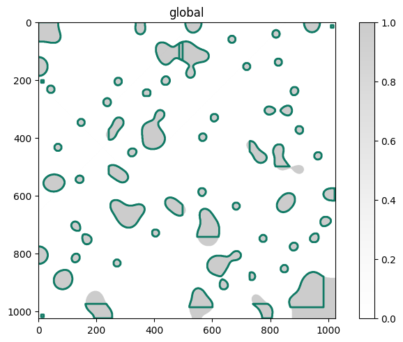
In a first step, we will load the spatialdata object and visualize the obtained cell segmentations (green outlines)

sdata = sd.read_zarr("./mock-data/blobs/sdata/my_sdata.zarr")
sdata

SpatialData object, with associated Zarr store: /Users/lucas-diedrich/Documents/Projects/scverse/spatialdata/spatialdata-io/dvp-io/dvp-io/docs/tutorials/mock-data/blobs/sdata/my_sdata.zarr
├── Images
│     └── 'blobs': DataArray[cyx] (1, 1024, 1024)
├── Points
│     └── 'calibration_points_image': DataFrame with shape: (<Delayed>, 2) (2D points)
└── Shapes
      └── 'segmentation_masks': GeoDataFrame shape: (62, 3) (2D shapes)
with coordinate systems:
    ▸ 'global', with elements:
        blobs (Images), calibration_points_image (Points), segmentation_masks (Shapes)
    ▸ 'to_lmd', with elements:
        segmentation_masks (Shapes)

(
    sdata.pl.render_images(cmap="Grays", alpha=0.2)
    .pl.render_shapes(fill_alpha=0, outline_color="#117A65", outline_width=2, outline_alpha=1)
    .pl.show(coordinate_systems="global")
)

The shapes are represented as a class:spatialdata.models.ShapesModel, which is in its core a class:geopandas.GeoDataFrame. class:geopandas.GeoDataFrames behave similarly to class:pandas.DataFrames. As you will see, this means that we can easily manipulate them to create selections of our for cells of interest.

assert isinstance(sdata.shapes["segmentation_masks"], gpd.GeoDataFrame)

Create selections

In the following, we will use three different selection criteria to select different cells:

1. A random selection of cells

2. A selection of cells based on a property (here: area)

3. A selection of cells based on their location in a region of interest (ROI)

Subsequently, we will write these subsets to an LMD-compatible .xml file.

Random selection

First, we will create a random selection of cells. This can be achieved with the built-in method gpd.GeoDataFrame.sample

# extract cell segmentation ShapesModel from spatialdata, create copy in memory
gdf = sdata.shapes["segmentation_masks"].copy()
# Get number of cell masks
len(gdf)

62

# Sample 10 cells, reassign them to sdata object
sdata.shapes["segmentation_masks_subset_random"] = gdf.sample(n=10, random_state=42)
len(sdata.shapes["segmentation_masks_subset_random"])

10

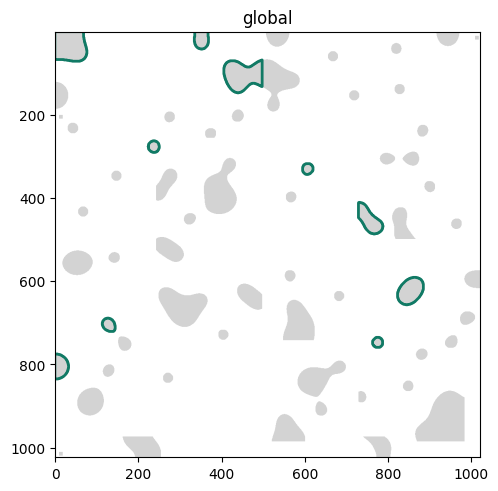
Cool! We selected exactly 10 shapes from the cell segmentation. Let’s visualize our random selection:

(
    sdata.pl.render_shapes("segmentation_masks")
    # Highlight only selected cell masks
    .pl.render_shapes(
        "segmentation_masks_subset_random", fill_alpha=0, outline_color="#117A65", outline_width=2, outline_alpha=1
    )
    .pl.show(coordinate_systems="global")
)

Selection based on property

We can also select cells based on a property. To do so, we will first compute the area of each segmented cell with the shapely function shapely.Polygon.area and assign it as new column to the ShapesModel. Subsequently, we will create a selection based on this property, following the well-known .loc logic.

# Copy ShapesModel
gdf = sdata.shapes["segmentation_masks"].copy()

# Compute and assign area (in Px^2) as new column
gdf["area"] = gdf["geometry"].apply(lambda geom: geom.area)
gdf

	name	well	geometry	area
0	Shape_1	None	POLYGON ((-0.603 0.518, -0.603 1.518, -0.603 2...	5009.0
1	Shape_2	None	POLYGON ((-0.603 120.518, -0.603 121.518, -0.6...	1670.5
2	Shape_3	None	POLYGON ((9.397 200.518, 9.397 201.518, 9.397 ...	81.0
3	Shape_4	None	POLYGON ((38.397 219.518, 37.397 220.518, 36.3...	518.0
4	Shape_5	None	POLYGON ((143.397 334.718, 142.397 335.718, 14...	471.0
...	...	...	...	...
57	Shape_58	None	POLYGON ((729.997 410.718, 728.997 411.718, 72...	2431.5
58	Shape_59	None	POLYGON ((824.997 422.718, 823.997 423.718, 82...	2631.5
59	Shape_60	None	POLYGON ((859.997 590.918, 858.997 591.918, 85...	2997.0
60	Shape_61	None	POLYGON ((944.997 863.118, 943.997 864.118, 94...	10771.5
61	Shape_62	None	POLYGON ((261.597 614.918, 260.597 615.918, 25...	7268.5

62 rows × 4 columns

We can visualize the areas as histograms

sns.histplot(gdf["area"])

<Axes: xlabel='area', ylabel='Count'>

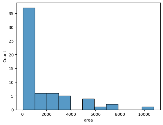
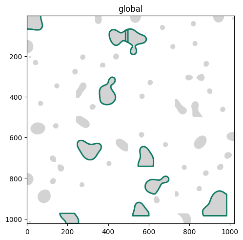
Let’s only select the 20 largest masks

gdf = gdf.nlargest(10, "area")
len(gdf)

10

And assign it as new attribute to the spatialdata object

sdata.shapes["segmentation_masks_subset_property"] = gdf

We can check again which shapes we selected

(
    sdata.pl.render_shapes("segmentation_masks")
    # Highlight only selected cell masks
    .pl.render_shapes(
        "segmentation_masks_subset_property", fill_alpha=0, outline_color="#117A65", outline_width=2, outline_alpha=1
    )
    .pl.show(coordinate_systems="global")
)

Selection based on region of interest

Lastly, we will select all cells that lie in a region of interest. First, we will define this area. Here, we will use napari to interactively define an area of interest.

## Uncomment the following lines for interactive ROI selection
# interactive = Interactive(sdata)
# interactive.run()

1. Create a new Shapes Layer

2. Select the rectangle tool

3. Select the area of interest

4. Save layer selection with Shift+E

Alternatively and for the purpose of reproducibility, you can use the following rectangle to the annotation layer:

roi = shapely.Polygon([[130, 173], [498, 173], [498, 477], [130, 477], [130, 173]])

sdata.shapes["roi"] = ShapesModel.parse(gpd.GeoDataFrame(geometry=[roi]))

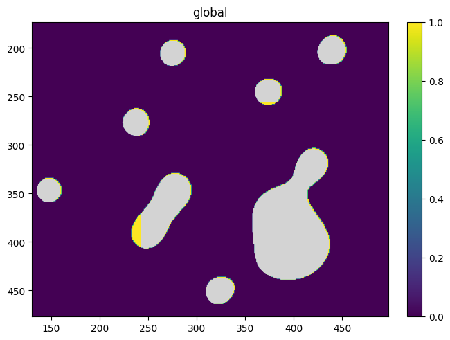
Next, we query the class:spatialdata.SpatialData object for this region of intest. The segmentation masks in this subset are automatically subsetted to the only the shapes within the region of interest:

roi = sdata.shapes["roi"].loc[0, "geometry"]
subset = sdata.query.polygon(roi, target_coordinate_system="global")

# Visualize the subset
subset.pl.render_images().pl.render_shapes("segmentation_masks").pl.show(coordinate_systems="global")

Lastly, we extract the associated shapes and assign them to our full spatialdata object

gdf = subset.shapes["segmentation_masks"]
sdata.shapes["segmentation_masks_subset_roi"] = gdf

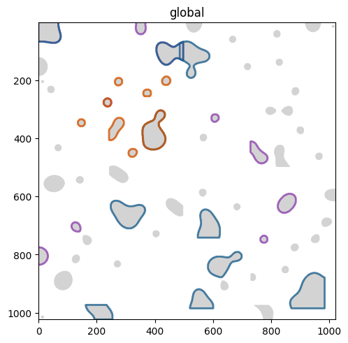
Visualize

Let’s visualize the shapes

(
    sdata.pl.render_shapes("segmentation_masks")
    # Highlight only selected cell masks
    .pl.render_shapes(
        "segmentation_masks_subset_random", fill_alpha=0, outline_color="#8E44AD", outline_width=2, outline_alpha=0.8
    )  # purple
    .pl.render_shapes(
        "segmentation_masks_subset_property", fill_alpha=0, outline_color="#1F618D", outline_width=2, outline_alpha=0.8
    )  # blue
    .pl.render_shapes(
        "segmentation_masks_subset_roi", fill_alpha=0, outline_color="#D35400", outline_width=2, outline_alpha=0.8
    )  # orange
    .pl.show(coordinate_systems="global")
)

Write

Finally, using dvp-io, we can write the selected shapes to a LMD-compatible .xml file. This represents a wrapper to the pylmd software package by Sophia Mädler et al., 2023

path_random = os.path.join(tempfile.tempdir, "pylmd-random-subset.xml")
# path_property = os.path.join(tempfile.tempdir, "pylmd-property-subset.xml")
# path_roi = os.path.join(tempfile.tempdir, "pylmd-roi-subset.xml")

write_lmd(
    path_random,
    sdata.shapes["segmentation_masks_subset_random"],
    calibration_points=sdata.points["calibration_points_image"],
)

[101500.  -1500.]
[20500. -1500.]
[   1500. -101500.]

Just for fun, we can inspect the head of the xml file

with open(path_random) as f:
    xml = f.read()

# Print head
print(xml[:697])

<?xml version='1.0' encoding='UTF-8'?>
<ImageData>
  <GlobalCoordinates>1</GlobalCoordinates>
  <X_CalibrationPoint_1>101500</X_CalibrationPoint_1>
  <Y_CalibrationPoint_1>-1500</Y_CalibrationPoint_1>
  <X_CalibrationPoint_2>20500</X_CalibrationPoint_2>
  <Y_CalibrationPoint_2>-1500</Y_CalibrationPoint_2>
  <X_CalibrationPoint_3>1500</X_CalibrationPoint_3>
  <Y_CalibrationPoint_3>-101500</Y_CalibrationPoint_3>
  <ShapeCount>10</ShapeCount>
  <Shape_1>
    <PointCount>129</PointCount>
    <X_1>51</X_1>
    <Y_1>-33560</Y_1>
    <X_2>151</X_2>
    <Y_2>-33560</Y_2>
    <X_3>251</X_3>
    <Y_3>-33560</Y_3>
    <X_4>351</X_4>
    <Y_4>-33560</Y_4>
    <X_5>451</X_5>
    <Y_5>-33560</Y_5>