Read DVP data into the spatialdata format

In this tutorial, we will read DVP data into the spatialdata format using DVP IO. We assume that cell segmentation was performed, e.g. in cellpose, and that the segmentation masks were processed and vectorized in BIAS and exported as LMD-compatible .xml files. We can now use spatialdata to further explore the data interactively, select shapes, etc.

Installation

## Uncomment the following lines if you still need to create a suitable environment etc.
# conda create -n dvpio python=3.11 -y && conda activate dvpio
# pip install dvp-io

Get data

We can get some mock data. Feel free to adjust the path to a suitable location

Dataset

The mock data contains an image, segmented shapes in the LMD .xml file format, and the ground truth for the generation of the shapes as .geojson for comparison.

• mock-data/blobs

  • images

    • binary-blobs.tiff

  • shapes

    • all_tiles_contours.xml

    • middle_tiles_contours.xml

  • ground_truth

    • binary-blobs.segmentation.geojson

# %%capture
# %%bash 
# downloadpath="./mock-data"
# mkdir -p $downloadpath 
# wget -O $downloadpath/blobs.zip "https://datashare.biochem.mpg.de/s/0oTGB6xpUaWIaVh/download"
# unzip -d $downloadpath $downloadpath/blobs.zip
# rm $downloadpath/blobs.zip

Read with DVP IO

We will now try to read in the data to the spatialdata format. This involves the following steps:

1. Generate spatialdata object

2. Read image

3. Read calibration points

4. Read segmentation masks and align via calibration points

5. Optional: Write spatialdata

import spatialdata
import spatialdata_plot  # noqa
from napari_spatialdata import Interactive  # noqa

from dvpio.read.image import read_custom
from dvpio.read.shapes import read_lmd

Initialize spatialdata

First, we initialize an empty spatialdata object

sdata = spatialdata.SpatialData()
sdata

SpatialData object
with coordinate systems:

Read image

Then, we read an image. In this case, we are dealing with a tiff file, so we will be using the dvpio.image.read_custom function that natively supports tiff images. The function parses the file directly into the spatialdata-compatible format, so that you can just add it to the spatialdata.image attribute

Alternative readers

If you were working with .czi files, you would instead use the read_czi reader function. Similarly, you would use the read_openslide reader for openslide compatible whole slide images.

img = read_custom("./mock-data/blobs/images/binary-blobs.tiff")
img

INFO     no axes information specified in the object, setting `dims` to: ('c', 'y', 'x')

<xarray.DataArray 'image' (c: 1, y: 1024, x: 1024)> Size: 8MB
dask.array<getitem, shape=(1, 1024, 1024), dtype=float64, chunksize=(1, 1024, 1024), chunktype=numpy.ndarray>
Coordinates:
  * c        (c) int64 8B 0
  * y        (y) float64 8kB 0.5 1.5 2.5 3.5 ... 1.022e+03 1.022e+03 1.024e+03
  * x        (x) float64 8kB 0.5 1.5 2.5 3.5 ... 1.022e+03 1.022e+03 1.024e+03
Attributes:
    transform:  {'global': Identity }

xarray.DataArray

'image'

• c: 1
• y: 1024
• x: 1024

• dask.array<chunksize=(1, 1024, 1024), meta=np.ndarray>

  Array Chunk Bytes 8.00 MiB 8.00 MiB Shape (1, 1024, 1024) (1, 1024, 1024) Dask graph 1 chunks in 2 graph layers Data type float64 numpy.ndarray

• Coordinates: (3)
  • c
    (c)
    int64
    0

    long_name :

    c

    units :

    array([0])

  • y
    (y)
    float64
    0.5 1.5 2.5 ... 1.022e+03 1.024e+03

    array([5.0000e-01, 1.5000e+00, 2.5000e+00, ..., 1.0215e+03, 1.0225e+03,
           1.0235e+03])

  • x
    (x)
    float64
    0.5 1.5 2.5 ... 1.022e+03 1.024e+03

    array([5.0000e-01, 1.5000e+00, 2.5000e+00, ..., 1.0215e+03, 1.0225e+03,
           1.0235e+03])

• Indexes: (3)
  • c
    PandasIndex

    PandasIndex(Index([0], dtype='int64', name='c'))

  • y
    PandasIndex

    PandasIndex(Index([   0.5,    1.5,    2.5,    3.5,    4.5,    5.5,    6.5,    7.5,    8.5,
              9.5,
           ...
           1014.5, 1015.5, 1016.5, 1017.5, 1018.5, 1019.5, 1020.5, 1021.5, 1022.5,
           1023.5],
          dtype='float64', name='y', length=1024))

  • x
    PandasIndex

    PandasIndex(Index([   0.5,    1.5,    2.5,    3.5,    4.5,    5.5,    6.5,    7.5,    8.5,
              9.5,
           ...
           1014.5, 1015.5, 1016.5, 1017.5, 1018.5, 1019.5, 1020.5, 1021.5, 1022.5,
           1023.5],
          dtype='float64', name='x', length=1024))

• Attributes: (1)

  transform :

  {'global': Identity }

We can now add the image to the spatialdata.images attribute

# Assign to spatialdata.images slot
sdata.images["blobs"] = img
sdata

SpatialData object
└── Images
      └── 'blobs': DataArray[cyx] (1, 1024, 1024)
with coordinate systems:
    ▸ 'global', with elements:
        blobs (Images)

Identify calibration points

To align the image with the segmented cells, we need to pick the calibration points in the image. We can do this interactively in the Napari Viewer.

The calibration points are small squares in the bottom left, top left, and top right corner of the image.

## Uncomment to run
# interactive = Interactive(sdata)
# interactive.add_element("blobs", element_coordinate_system="global")
# interactive.run()

Picking calibration points

1. Create a new points layer in the napari viewer.

2. Recommended: Rename the layer to a more expressive name, e.g. calibration_points_image

3. Select the 3 calibration points. Currently, you have to pick them in the correct order, as they are defined in the lmd/.xml file. (Here: 1. bottom left, 2. top left, 3. top right)

4. Save the layer by clicking Shift+E

5. Leave the napari viewer.

The calibration points were added to the shapes attribute of the spatialdata object

# Uncomment to assign ground truth values
import numpy as np

sdata.points["calibration_points_image"] = spatialdata.models.PointsModel.parse(
    np.array([[15, 1015], [15, 205], [1015, 15]])
)

sdata

SpatialData object
├── Images
│     └── 'blobs': DataArray[cyx] (1, 1024, 1024)
└── Points
      └── 'calibration_points_image': DataFrame with shape: (<Delayed>, 2) (2D points)
with coordinate systems:
    ▸ 'global', with elements:
        blobs (Images), calibration_points_image (Points)

Read segmentation masks from LMD .xml

You can now load the segmentation masks from the LMD formatted .xml file, using the designated read_lmd function. The function returns a geopandas.GeoDataFrame that can be immediately passed to the spatialdata.shapes attribute

sdata.shapes["segmentation_masks"] = read_lmd(
    "./mock-data/blobs/shapes/all_tiles_contours.xml",
    calibration_points_image=sdata.points["calibration_points_image"],
    switch_orientation=False,
)

sdata.shapes["segmentation_masks"]

	name	well	geometry
0	Shape_1	None	POLYGON ((-0.603 0.518, -0.603 1.518, -0.603 2...
1	Shape_2	None	POLYGON ((-0.603 120.518, -0.603 121.518, -0.6...
2	Shape_3	None	POLYGON ((9.397 200.518, 9.397 201.518, 9.397 ...
3	Shape_4	None	POLYGON ((38.397 219.518, 37.397 220.518, 36.3...
4	Shape_5	None	POLYGON ((143.397 334.718, 142.397 335.718, 14...
...	...	...	...
57	Shape_58	None	POLYGON ((729.997 410.718, 728.997 411.718, 72...
58	Shape_59	None	POLYGON ((824.997 422.718, 823.997 423.718, 82...
59	Shape_60	None	POLYGON ((859.997 590.918, 858.997 591.918, 85...
60	Shape_61	None	POLYGON ((944.997 863.118, 943.997 864.118, 94...
61	Shape_62	None	POLYGON ((261.597 614.918, 260.597 615.918, 25...

62 rows × 3 columns

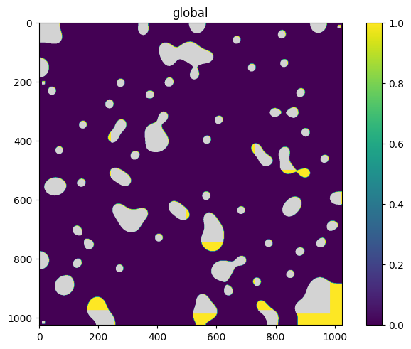
We can now inspect the results as static images or in a dynamic Napari session. We see that the segmentation masks and blobs overlay reasonably well.

sdata.pl.render_images("blobs").pl.render_shapes("segmentation_masks").pl.show(coordinate_systems="global")

Write

If you would like to keep a persistent copy of your spatialdata object on disk, use the write functionality:

sdata.write("./mock-data/blobs/sdata/my_sdata.zarr")

INFO     The Zarr backing store has been changed from None the new file path: mock-data/blobs/sdata/my_sdata.zarr