Real-world example - Analysis of scDVP liver zonation dataset

In this example we showcase how spatialdata can be leveraged in the analysis of real-world DVP data. For this purpose we utilize a small subset of the previously published dataset by [RTS+23] (Rosenberger et al, 2023), specifically the sample m1a. This datasets includes

• IF images (as .tiff) of the mouse liver, including the markers Glutamine Synthethase, E-Cadherin, cell membrane marker (WGA), and phalloidin (cytoskeleton)

• Cell segmentation shapes of the profiled cells as LMD-compatible .xml file

• Proteomics measurements of 77 single shapes as diann protein groups report (.tsv)

We will see how we can use spatialdata to jointly store and visualize these different modalities.

Packages

To process the different modalities, we import the respective readers from dvpio (see the FAQ) for a full list of available readers). Additionally, we will import some scientific software packages, including spatialdata

import numpy as np
import pandas as pd

import matplotlib as mpl
import matplotlib.pyplot as plt

import spatialdata as sd
import spatialdata_plot  # noqa

from dvpio.read.image import read_custom
from dvpio.read.omics import parse_df
from dvpio.read.shapes import read_lmd

Get data

# %%capture
# %%bash
# downloadpath="./scdvp"
# mkdir -p $downloadpath
# wget -O $downloadpath/scdvp-rosenberger2023.zip "https://datashare.biochem.mpg.de/s/Z0BBq65fFHX3ai3/download"
# unzip -d $downloadpath $downloadpath/scdvp-rosenberger2023.zip
# rm $downloadpath/scdvp-rosenberger2023.zip

image_path = "./scdvp/images"
lmd_path = "./scdvp/shapes/EXP-220815_m1A_plate-2.pylmd.xml"
protein_group_df_path = "./scdvp/omics/PXD038699_proteintable.tsv"

Create spatialdata object

We will successively add attributes to our spatialdata object. Let’s initialize an empty object:

sdata = sd.SpatialData()

Load images

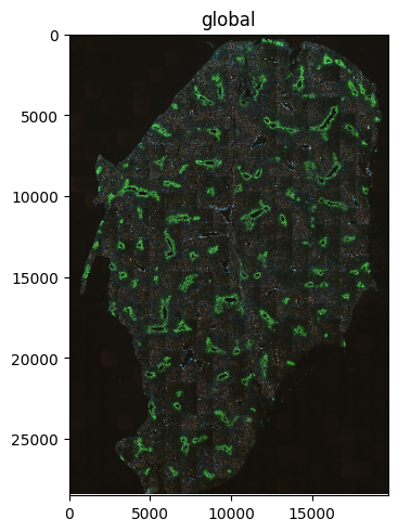
First, we will add the tiff images using the respective dvpio function and visualize it

sdata.images["m1a_image"] = read_custom(path=f"{image_path}/S-BIAD596_m1A_*.tif")

INFO     no axes information specified in the object, setting `dims` to: ('c', 'y', 'x')

norm = mpl.colors.Normalize(vmin=0, vmax=4000)
sdata.pl.render_images("m1a_image", norm=norm).pl.show()

INFO     Rasterizing image for faster rendering.

Load shapes

Next, we load the shapes. To do this, we will first need to define the calibration points in the image. As the calibration points are not visible in the image, we pass the values that were used in the original publication (link). Alternatively, you can also interactively select the points with napari_spatialdata, see Tutorial 2

# Calibration points were determined at 0.135545805x resolution in a coordinate system that was centered at the image center
# + we need to scale them to 1x resolution (x1/0.135545805)
# + shift the coordinate system to the upper left corner of the image (+image width/2, image width/2)
url = "https://raw.githubusercontent.com/MannLabs/single-cell-DVP/cf9d588849f84409c2e0ce6e3703cc69a1823503/data/meta/coordinates_meta.txt"
df = pd.read_csv(url, sep="\t")
df["X_scaled"] = df["X"] / df["resolution"]
df["Y_scaled"] = df["Y"] / df["resolution"]
df["X_transformed"] = df["X_scaled"] + sdata.images["m1a_image"].shape[2] / 2
df["Y_transformed"] = df["Y_scaled"] + sdata.images["m1a_image"].shape[1] / 2

calibration_points_image = df.loc[df["Slide"] == "m1A", ["X_transformed", "Y_transformed"]].values

sdata.points["calibration_points_image"] = sd.models.PointsModel.parse(calibration_points_image)

calibration_points_image

array([[ 1836.11676551,  9121.12330304],
       [18291.61238192,  3189.23998138],
       [ 7121.62375704, 25625.42677448]])

Having defined the calibration points, we can now read the actual shapes from the LMD-compatible .xml file and add them to spatialdata.

sdata.shapes["cell_segmentation"] = (
    read_lmd(
        lmd_path,
        calibration_points_image=sdata.points["calibration_points_image"],
        transformation_type="similarity",
        precision=6,
    )
    .set_index("name", drop=False)
    .rename_axis(None, axis=0)
)

You should always check/validate whether cell segmentation and image are correctly overlaid. To do so, we select a small subset of the image and take a look at both cell membrane staining (channel 1) and cell segmentation

fig, ax = plt.subplots(1, 1, figsize=(8, 5))

min_coordinate = np.array([6200, 6600])
max_coordinate = min_coordinate + 700

(
    sdata.query.bounding_box(
        axes=("x", "y"),
        min_coordinate=min_coordinate,
        max_coordinate=max_coordinate,
        target_coordinate_system="global",
    )
    .pl.render_images("m1a_image", channel=1)
    .pl.render_shapes(fill_alpha=0.0, outline_alpha=1, outline_color="#efefef")
    .pl.show(coordinate_systems="global", ax=ax)
)

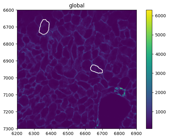
The overlay between shapes and cell membrane stain looks reasonable.

Omics data

Finally, we add the omics data. In this case, we start from the protein.group dataframe as reported by DIANN (source) and use the :func:dvpio.read.omics.parse_df function to parse the data into a spatialdata-compatible anndata.AnnData container.

Note, that the function expects a processed version of the dataframe: Cell-level metadata must be stored in the dataframe row index and will be stored in the anndata.AnnData.obs attribute. Gene-level metadata must be stored in the dataframe columns index and will be stored in the anndata.AnnData.var attribute. All values of the dataframe will be stored in anndata.AnnData.X.

# Read DIANN Report
df = pd.read_csv(protein_group_df_path, sep="\t", index_col="protein").T.reset_index(names="run")

# Parse metadata run into individual metadata columns
metadata_columns = [
    "date",
    "ms",
    "A",
    "B",
    "C",
    "method",
    "sample_id",
    "uniprot_ref",
    "aid",
    "cell_id",
    "D",
    "E",
    "F",
    "G",
]
df[metadata_columns] = df["run"].str.split("_").tolist()

# Create new metadata column `name` that matches the shape names in in the cell segmentation
df["name"] = df["cell_id"].apply(lambda x: f"Shape_{int(x)}")

# Add metadata column that enables spatialdata to match the measurements
# to the cell segmentation shapes (stored in sdata.shapes["cell_segmentation"]) [expects name of shapes attribute]
df["region_key"] = "cell_segmentation"

# Subset to unique cells
# TODO discuss why there are multiple measurements per cell
df = df.groupby("name").first().reset_index()

# Set all metadata columns, including the newly generated ones to the dataframe index
df = df.set_index(["run", "name", "region_key", *sorted(metadata_columns)])

df

																protein	A0A087WQ94	A0A087WR50	A0A087WSP5	A0A0A6YVS2	A0A0A6YW80	A0A0J9YU79	A0A0J9YUI8	A0A0R4IZY2	A0A0R4J083	A0A0R4J0B4	...	P54726	Q61581	Q3V2R3	Q6S9I0	Q9D0J4	Q99N93	Q8CHY6	P11835	P56183	Q6P8J7
run	name	region_key	A	B	C	D	E	F	G	aid	cell_id	date	method	ms	sample_id	uniprot_ref
20220820_TIMS06_FAS_SA_S720_scDVP_m1A_Ref10_AID8_01_S2-A1_1_4970_target4	Shape_1	cell_segmentation	FAS	SA	S720	S2-A1	1	4970	target4	AID8	01	20220820	scDVP	TIMS06	m1A	Ref10	2546.170495	3112.807142	4247.124853	1906.437899	4825.246524	1589.062179	736.197798	6044.616609	6140.588482	1625.809065	...	NaN	NaN	NaN	NaN	NaN	NaN	NaN	NaN	NaN	NaN
20220820_TIMS06_FAS_SA_S720_scDVP_m1A_Ref10_AID8_10_S2-A10_1_4979_target4	Shape_10	cell_segmentation	FAS	SA	S720	S2-A10	1	4979	target4	AID8	10	20220820	scDVP	TIMS06	m1A	Ref10	8077.136135	3330.472828	2268.027890	1526.827577	6940.136352	3275.123797	2150.213041	10486.206852	6641.898142	12554.911721	...	NaN	NaN	NaN	NaN	NaN	NaN	NaN	NaN	NaN	NaN
20220820_TIMS06_FAS_SA_S720_scDVP_m1A_Ref10_AID8_11_S2-A11_1_4980_target4	Shape_11	cell_segmentation	FAS	SA	S720	S2-A11	1	4980	target4	AID8	11	20220820	scDVP	TIMS06	m1A	Ref10	NaN	4435.863428	5348.012649	1748.762739	10268.052605	1197.900908	2981.050155	12238.028228	8792.139128	1203.145811	...	NaN	NaN	3487.29117	NaN	NaN	NaN	NaN	NaN	NaN	NaN
20220820_TIMS06_FAS_SA_S720_scDVP_m1A_Ref10_AID8_12_S2-B1_1_4981_target8	Shape_12	cell_segmentation	FAS	SA	S720	S2-B1	1	4981	target8	AID8	12	20220820	scDVP	TIMS06	m1A	Ref10	1196.769924	3220.892955	5649.794082	5531.072645	11462.061995	1891.362297	3109.722352	8266.772895	4655.184605	3886.250550	...	NaN	NaN	NaN	NaN	NaN	NaN	NaN	NaN	NaN	NaN
20220820_TIMS06_FAS_SA_S720_scDVP_m1A_Ref10_AID8_13_S2-B2_1_4982_target8	Shape_13	cell_segmentation	FAS	SA	S720	S2-B2	1	4982	target8	AID8	13	20220820	scDVP	TIMS06	m1A	Ref10	3896.896268	3892.945494	3787.335743	3654.229206	9770.141567	2570.591653	3336.025993	13528.636038	8340.092785	2791.022612	...	NaN	318.401047	NaN	NaN	NaN	NaN	NaN	NaN	NaN	NaN
...	...	...	...	...	...	...	...	...	...	...	...	...	...	...	...	...	...	...	...	...	...	...	...	...	...	...	...	...	...	...	...	...	...	...	...	...	...
20220820_TIMS06_FAS_SA_S720_scDVP_m3B_Ref10_AID8_75_S2-G9_1_4961_target4	Shape_75	cell_segmentation	FAS	SA	S720	S2-G9	1	4961	target4	AID8	75	20220820	scDVP	TIMS06	m3B	Ref10	1853.740651	3846.307917	2964.671425	3770.539387	6331.494696	4519.779519	2492.729865	15927.070502	11184.127594	232.821475	...	NaN	NaN	NaN	NaN	NaN	NaN	NaN	NaN	NaN	1078.283601
20220820_TIMS06_FAS_SA_S720_scDVP_m3B_Ref10_AID8_76_S2-G10_1_4962_target4	Shape_76	cell_segmentation	FAS	SA	S720	S2-G10	1	4962	target4	AID8	76	20220820	scDVP	TIMS06	m3B	Ref10	4479.211592	2225.215970	3729.255133	1500.205313	20813.766732	5020.883312	2230.125342	8551.449242	5701.956014	1810.053280	...	NaN	NaN	NaN	NaN	NaN	NaN	NaN	NaN	NaN	NaN
20220820_TIMS06_FAS_SA_S720_scDVP_m3B_Ref10_AID8_77_S5-G11_1_4963_target8	Shape_77	cell_segmentation	FAS	SA	S720	S5-G11	1	4963	target8	AID8	77	20220820	scDVP	TIMS06	m3B	Ref10	3994.153689	2295.307398	2192.080927	15405.786639	1908.038186	3279.212194	2958.605514	7308.751211	4870.938330	1780.867609	...	NaN	NaN	NaN	NaN	488.112002	NaN	NaN	NaN	NaN	NaN
20220820_TIMS06_FAS_SA_S720_scDVP_m1A_Ref10_AID8_08_S2-A8_1_4977_target4	Shape_8	cell_segmentation	FAS	SA	S720	S2-A8	1	4977	target4	AID8	08	20220820	scDVP	TIMS06	m1A	Ref10	3880.901353	3354.038617	3288.165942	3010.736507	5709.819890	3183.414270	2314.839162	16373.762603	11374.528812	3555.521124	...	NaN	NaN	NaN	NaN	NaN	NaN	NaN	NaN	NaN	NaN
20220820_TIMS06_FAS_SA_S720_scDVP_m1A_Ref10_AID8_09_S2-A9_1_4978_target8	Shape_9	cell_segmentation	FAS	SA	S720	S2-A9	1	4978	target8	AID8	09	20220820	scDVP	TIMS06	m1A	Ref10	3086.943355	3421.335838	2606.051069	5119.567885	9104.939493	2330.939112	2840.631062	11393.620934	5431.817081	2077.488892	...	173.200087	480.249257	NaN	NaN	NaN	NaN	NaN	NaN	NaN	NaN

77 rows × 3738 columns

# Parse dataframe
# Set anndata.AnnData.var index to protein uniprot accessors to enable querying by protein names (required for plotting)
sdata.tables["m1a_table"] = parse_df(
    df, var_index="protein", region="cell_segmentation", region_key="region_key", instance_key="name"
)
# Inspect
sdata.tables["m1a_table"]

AnnData object with n_obs × n_vars = 77 × 3738
    obs: 'run', 'name', 'region_key', 'A', 'B', 'C', 'D', 'E', 'F', 'G', 'aid', 'cell_id', 'date', 'method', 'ms', 'sample_id', 'uniprot_ref'
    uns: 'spatialdata_attrs'

After having added the omics layer to the spatialdata object, we can overlay the proteomics measurement with the imaging. In this example, we will focus on E-Cadherin (P09803) for which the original authors also developed an antibody-based staining.

min_coordinate = np.array([4000, 8000])
size = 5000

(
    sdata
    # Subset to relevant area
    .query.bounding_box(
        axes=("x", "y"),
        min_coordinate=min_coordinate,
        max_coordinate=min_coordinate + size,
        target_coordinate_system="global",
    )
)

SpatialData object
├── Images
│     └── 'm1a_image': DataArray[cyx] (4, 5000, 5000)
├── Shapes
│     └── 'cell_segmentation': GeoDataFrame shape: (11, 3) (2D shapes)
└── Tables
      └── 'm1a_table': AnnData (2, 3738)
with coordinate systems:
    ▸ 'global', with elements:
        m1a_image (Images), cell_segmentation (Shapes)
    ▸ 'to_lmd', with elements:
        cell_segmentation (Shapes)

sdata.tables["m1a_table"].obs["expression"] = sdata.tables["m1a_table"][:, "P09803"].X.flatten()

fig, axs = plt.subplots(1, 2, figsize=(16, 5))

min_coordinate = np.array([4000, 7000])
max_coordinate = min_coordinate + 600

(
    sdata
    # Subset to relevant area
    .query.bounding_box(
        axes=("x", "y"),
        min_coordinate=min_coordinate,
        max_coordinate=max_coordinate,
        target_coordinate_system="global",
    )
    .pl.render_images("m1a_image", channel=1)
    .pl.render_shapes(
        element="cell_segmentation", color="P09803", norm=mpl.colors.Normalize(0, 7000), outline_alpha=1, fill_alpha=1
    )
    .pl.show(coordinate_systems="global", ax=axs[0])
)

axs[0].set_title("LC/MS-measurement + $\\alpha$-E-Cadherin")

(
    sdata
    # Subset to relevant area
    .query.bounding_box(
        axes=("x", "y"),
        min_coordinate=min_coordinate,
        max_coordinate=max_coordinate,
        target_coordinate_system="global",
    )
    .pl.render_images("m1a_image", channel=1)
    .pl.render_shapes(
        element="cell_segmentation", color="P09803", outline_alpha=1, outline_color="#cccccc", fill_alpha=0
    )
    .pl.show(coordinate_systems="global", ax=axs[1])
)

axs[1].set_title("Cell segmentation + $\\alpha$-E-Cadherin")

Text(0.5, 1.0, 'Cell segmentation + $\\alpha$-E-Cadherin')

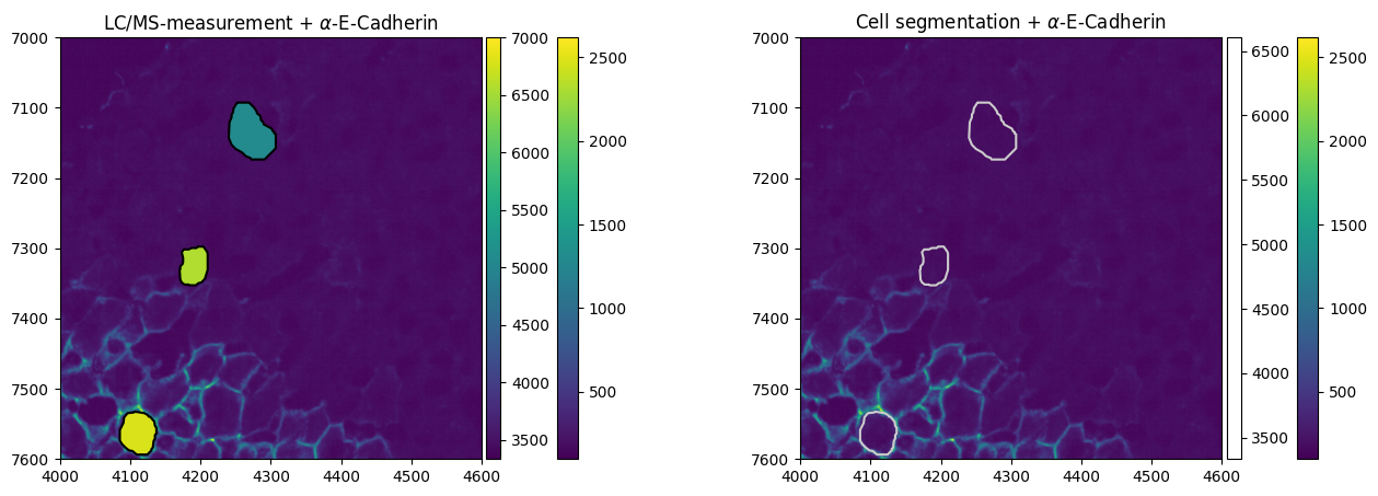
We note that the staining intensity correlates with the measured abundance of E-Cadherin in the cells.